Testing QSI's 532ws Scientific CCD Cameraby Richard Berry |
||||||||||||||
Originally published
in Astronomy Technology Today
magazine, Vol. 2, Issue 2, February 2008 |
||||||||||||||
| I wrote this
story for savvy amateur astronomers who are looking for a
top-notch CCD camera that is suitable for both imaging
and science purposes, especially if you want a
high-quality camera that seems to help you make great
images. Since I’ve been involved with CCD cameras
for quite some time, I’m amazed at the number of
fine imaging cameras available to amateurs on the market
today. But this story is about just one: Quantum
Scientific Imaging’s 532ws CCD camera. Our tale begins at the Society for Astronomical Sciences meeting, held each year before RTMC in Big Bear, CA, when I met Kevin Nelson. Kevin is a founder and the marketing director for Quantum Scientific Imaging. In the vendor area, Kevin was showing his company’s new line of scientific imaging cameras. He pulled out a notebook and proudly showed me the Fourier Transform of a bias frame—and that really got my attention. Why? Because bias frames are sensitive to system noise and Fourier Transforms reveal every problem—and he was showing results from an internal engineering test. Customers usually don’t get to see things like that. I was impressed. Kevin picked up on my interest, and asked whether I would be willing to test and evaluate the new 532ws camera. As the company’s name implies, QSI makes CCD cameras for scientific research, so I figured their products had to be reasonable good. And because I realized that Kevin actually wanted me to do a serious and demanding evaluation of the new camera, I agreed to do so. |
||||||||||||||
The QSI 532ws Arrives |
||||||||||||||
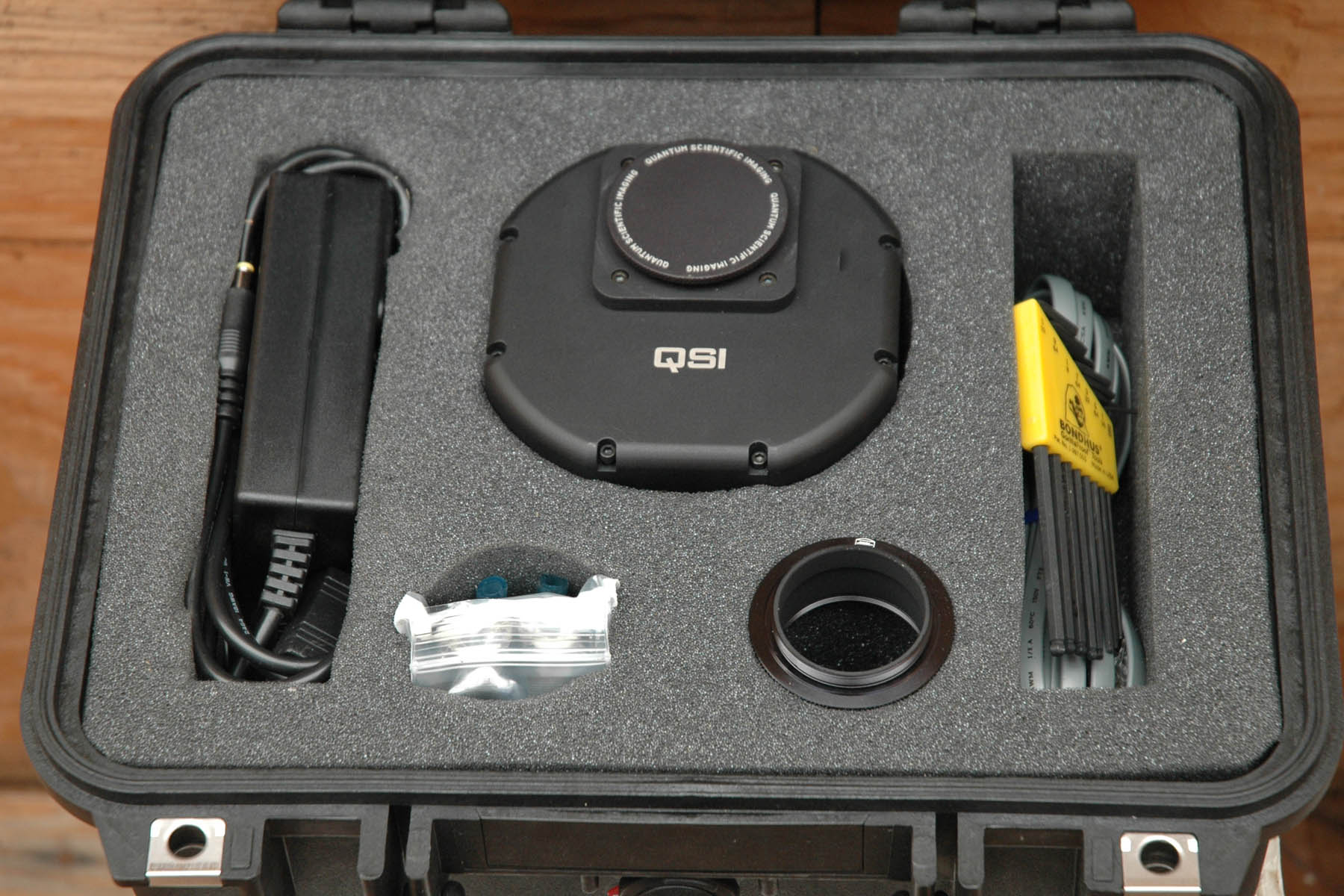
| The test camera arrived in mid-July. My initial impression on receiving the camera was extremely positive. It arrived in a sturdy double box, inside which was an airtight Pelican case containing the test camera (S/N#502137), power supply, USB 2.0 and guider cables, a T-mount to 2-inch adaptor, a set of Allen keys, plus an optional liquid heat exchanger for summertime cooling. Everything was snugly bedded in foam cutouts (Figure 1). QSI’s 532ws camera is based on Kodak’s 3.2-megapixel KAF-3200ME CCD. This CCD has 6.8-micron square pixels in a 2184 by 1472 array, and boasts a peak quantum efficiency of 80% or higher. The camera was configured to make images with an overscan area, common in science data cameras but rare in amateur imaging cameras. By now you are probably wondering why, as an amateur astronomer, I wanted to test a “science” camera? The answer is that because scientific applications demand more from a CCD than amateur imaging, I expected better overall performance. Amateur cameras can be noisy and display rather severe faults before those faults seriously interfere with making pictures of the Orion Nebula—but a scientific imaging camera has to meet a higher standard. I wanted a camera that would do a good job on really faint objects, that offered professional-quality firmware and electronics, a camera that would never stand in the way of taking great data or making great images. The test camera was a model 532ws. QSI offers the 532 in two types, the 532s (with mechanical shutter), and the 532ws (with mechanical shutter and five-position internal color filter wheel). The filter wheel in the test camera came populated with Astronomik LRGB Type IIc color filters. In size, the 532ws is 4½ by 4½ inches and 2½ inches deep; the 532s is somewhat thinner. On one side are the power, USB 2.0, and guider control sockets. You can see specifications for all of QSI’s cameras at http://www.qsimaging.com/. Setup went smoothly. Speaking as a professional writer/editor, I would award the manual that came with the 532ws the highest marks for clarity. It is well written, nicely illustrated, and complete. Using it as a guide, someone who had never set up and used a CCD camera before would probably encounter no problems. You can download the manual from QSI’s website; it’s a 2.0 MB PDF document. The arrival of the camera brought with it a lengthy spell of cloudy weather—perfect weather for testing! I set up the camera indoors and shot hundreds of bias frames, dark frames, and light-box flat-field frames. These would allow me to measure the camera’s basic performance characteristics (see the sidebar: Performance Testing a CCD Camera). |
||||||||||||||
Gain, Readout Noise, and Dark Current |
||||||||||||||
| Three numbers
tell you a lot about how a CCD camera performs. These are
the gain, readout noise, and dark current. They were the
first things I measured. The camera manufacturer sets the gain to maximize camera performance; you need to know the gain to convert pixel values in your images to the number of detected photons. The CCD adds readout noise; the lower it is, the better. And dark current is a parasitic signal generated by the CCD itself; lower is better. In The Handbook for Astronomical Image Processing (by me and Jim Burnell, published by Willmann-Bell, Inc. at http://www.willbell.com) we devoted a chapter (“Measuring CCD Performance”) to this subject, so I won’t repeat the technical details here. Suffice it to say that by taking two bias frames, two flat frames, and one long-exposure dark frame, anyone can determine the gain, the readout noise, and the dark current of a CCD camera. Furthermore, The Handbook for Astronomical Image Processing comes with full-featured processing software, Astronomical Image Processing for Windows, called AIP4Win for short. AIP4Win includes a CCD Calibration Tool so you don’t need to struggle through the math. Simply select the bias, flats, and dark frame, then click to get your results. The gain of the test camera was 1.33 electrons per ADU, its readout noise was 10.5 electrons r.m.s., and the average dark current of 0.08 electrons per pixel per second at an operating temperature of 0 Celsius. These are excellent figures. Kodak specifies a readout noise between 7 and 12 electrons r.m.s. for the KAF-3200ME, so the QSI camera and Kodak CCD met Kodak’s specifications. I’ll say more about dark current later in this story; suffice it to say here that dark frames turned out to be much more interesting—and very much better—than I anticipated. Once you have the gain and readout noise, you can calculate two more basic parameters: the saturation signal and the dynamic range. Saturation occurs when the count in ADU reaches 65,535. Kodak’s specified minimum for the saturation signal in electrons is 50,000 electrons; the test camera reached saturation at 49,300 electrons. I queried QSI about this: to accommodate the capacity of the horizontal shift register for 2x2 binning, QSI sets the gain somewhat high to provide the optimum tradeoff between saturation and dynamic range when the CCD is binned. This engineering decision benefits amateur astronomers shooting color images, and it does not significantly compromise Kodak’s saturation specification. Dynamic range is the ratio between the maximum signal and the readout noise; in the test camera the ratio was 4930:1. Engineers sometimes think in decibels; in the test camera, the dynamic range is 73.8 dB, that is, better than Kodak’s specification of 72 dB. Well, that’s a lot of numbers—gain, readout noise, dark current, saturation signal, and dynamic range! By measuring them the first day I had the camera, I did what any professional astronomer would have done: I had characterized the camera. By the end of the first day, I knew that the QSI camera and its KAF-3200ME CCD met specifications, and were likely to perform very well on the stars. After working with the evaluation QSI 532ws for another ten weeks, I ordered one for myself. When mine arrived (S/N#502314), the first thing I did was measure the basic parameters: they came out almost identical to those of the test camera. Shortly after that, a friend received his QSI 532ws, and it tested out with the same basic parameters. I must say that I am impressed with consistency of QSI’s product, and personally very pleased that my own camera tests every bit as good as the evaluation camera. |
||||||||||||||
Analysis of QSI 532ws Bias Frames |
||||||||||||||
| With the basic
parameters established, I began testing in earnest. While
the bad weather continued, I shot hundreds of bias
frames, dark frames, and flat frames. I’ll talk
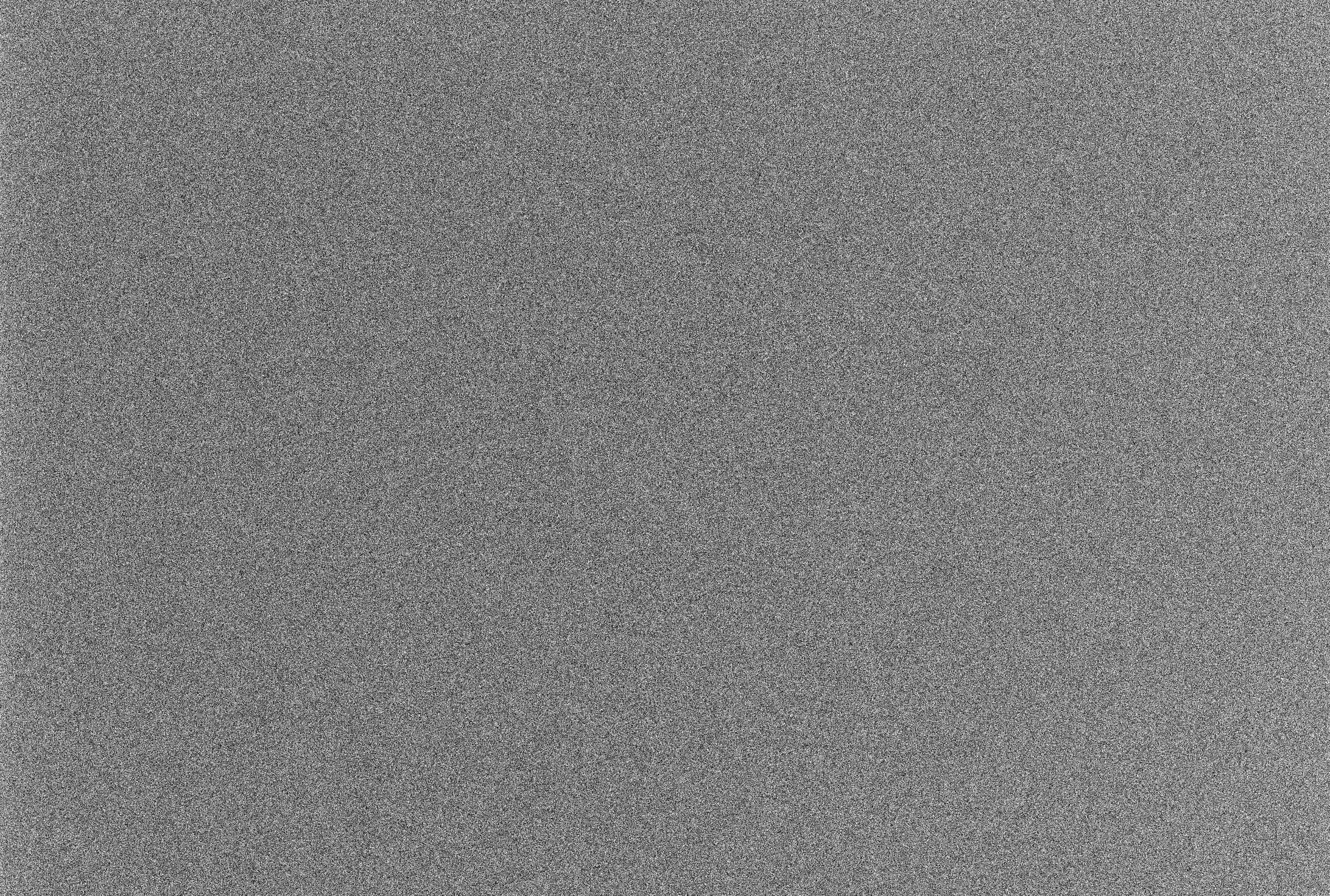
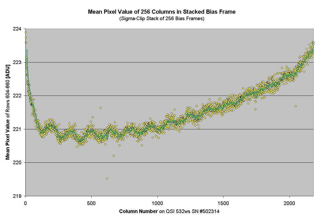
about the bias frames first. Bias frames reveal subtle aspects of a camera's "personality" that make a big difference when you try to take images at the limit. Bias frames are exquisitely sensitive to noise from faulty camera electronics, poor shielding from radiofrequency interference, faulty grounding, and a host of other problems. And if noise appears in the bias frame, you can be sure that every image you shoot—darks, flats, and images—will be noisy, too. What impressed me in looking over the mass of data I collected is that the QSI 532ws’ images are exceptionally clean and free of readout artifacts. Because I write image-processing software and collect sample images whenever I can, I’ve seen bias frames from many different CCD cameras. Bias frames should be perfectly flat, showing no features at all except random pixel-to-pixel variation due to readout noise. In reality, many cameras produce bias frames with quasi-random horizontal stripes, vertical patterns, plus a few (or sometimes many) dark or light columns. Taken together, these artifacts are called pattern noise. In some cameras, the pattern is the same in every bias frame; in other, the pattern is different in every bias frame. Repeating pattern noise is better than changing pattern noise, but all pattern noise is bad. Pattern noise points to shortcuts or unsolved problems in the design or construction of the CCD camera. However, the QSI 532ws’ bias frames looked so close to ideal that I was amazed. Figure 2 shows a typical bias frame. Histogram of bias frames show pure Gaussian noise with a standard deviation of 10.5 electrons r.m.s., that is, they showed pure random readout noise. However, I was not satisfied to say the bias frames from the QSI 532ws were perfect. After all, every dog has some fleas. To beat down readout noise and reveal whatever tiny residual pattern noise might be present, I combined hundreds of bias frames. The sigma-clipped mean of 256 bias frames appears in Figure 3. In the figure, readout noise has been reduced to about 0.65 electrons r.m.s. You can see the pattern noise as a subtle vertical fluting. By averaging 256 rows, I measured semi-random patterns to have an amplitude of 0.2 electrons, or about 2% of the readout noise, as shown in Figure 4. This is remarkably small compared to anything that I’ve seen in bias frames from other cameras; in some, the pattern noise is larger than readout noise. Having found and measured this tiny residual, I can say that for all practical intents and purposes, the test QSI 532ws bias frames are textbook perfect. And when my own 532ws arrived, its bias frames were just as good. I mentioned earlier that the QSI 532ws test camera was configured with an overscan area. In science cameras, an overscan area is included because it provides valuable insight into the operation of the camera and CCD. After clocking out the image area of the CCD, the electronics stop clocking the vertical shift registers but continue to clock the horizontal shift register. In the test camera, there were an additional 400 columns on the right-hand side of the image. These columns have lower pixel values and less noise than the area of the bias frame read from the image area of CCD. The random variation in the overscan is actually the “true” readout noise; it measured 8.1 electrons r.m.s. in the test camera (versus 10.5 electrons r.m.s. in the image area). This puts the “true” readout noise in the test camera at the low end of Kodak’s specified range of 7 to 12 electrons r.m.s. While measuring large numbers of bias frames, I noticed that the mean value of the entire image sometimes changed by plus or minus one ADU. This is quantization noise. It comes about because the analog signal from the CCD’s on-chip amplifier is converted to an integer value, and then auto-zeroed to a fixed value. Quantization noise adds approximately 0.5 electrons r.m.s. of random noise to the signal, and auto-zeroing quantization noise is present only when you combine a large number of images. Quantization noise is present in all digital imaging systems. In the QSI 532ws, quantization noise (0.5 electrons r.m.s.) is negligibly small compared to readout noise (10.5 electrons r.m.s.) and shot noise (often a few hundred electrons r.m.s.). I detected quantization noise only because I set out to measure every source of noise I could find. |
||||||||||||||
Analysis of QSI 532ws Dark Frames and Dark Current |
||||||||||||||
| To investigate
the QSI 532ws’ dark current, on cloudy nights I shot
bias and dark frames at temperatures ranging from 0
Celsius to -25 Celsius with exposure times ranging from
10 seconds to 1000 seconds. This produced many gigabytes
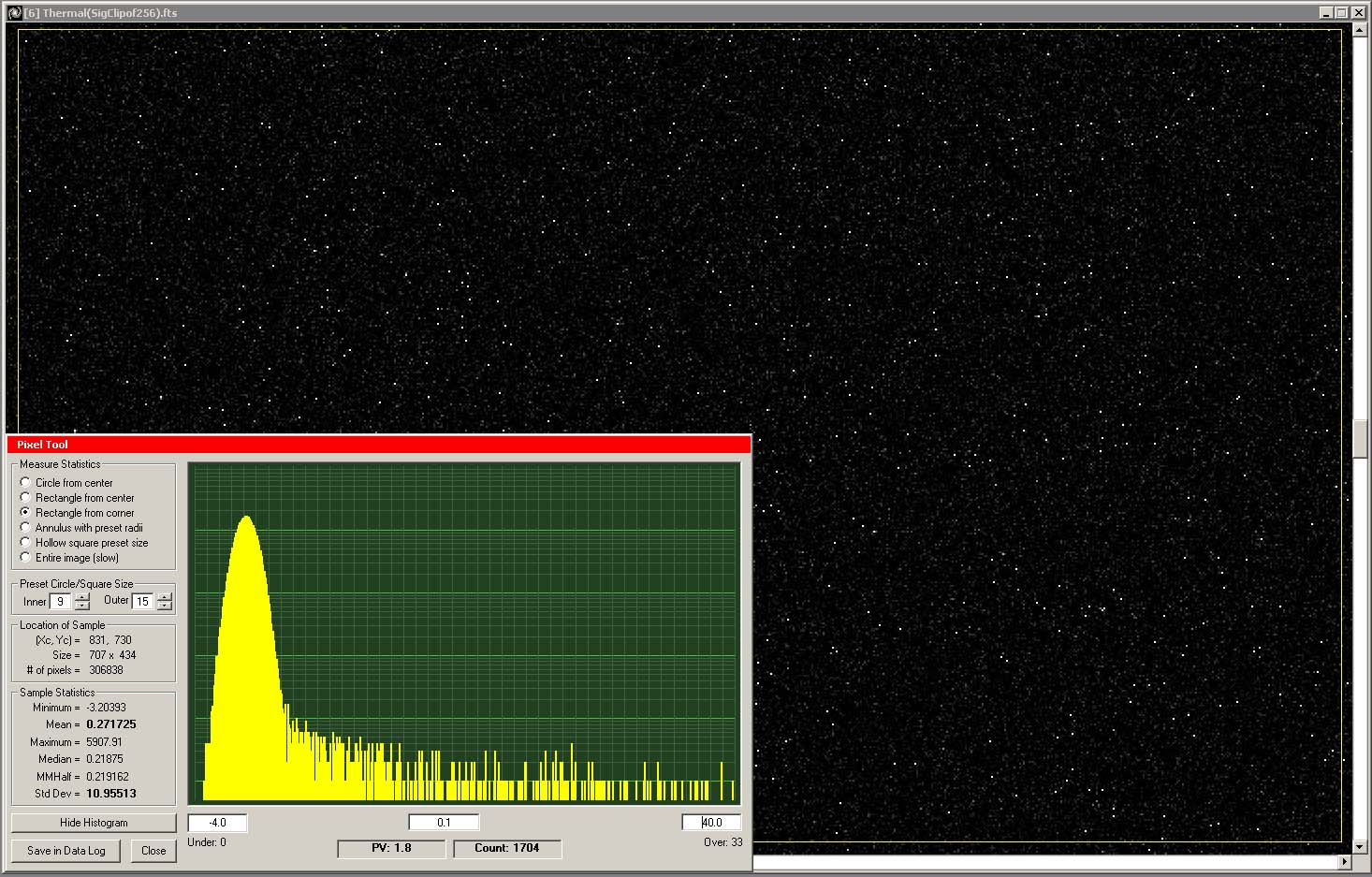
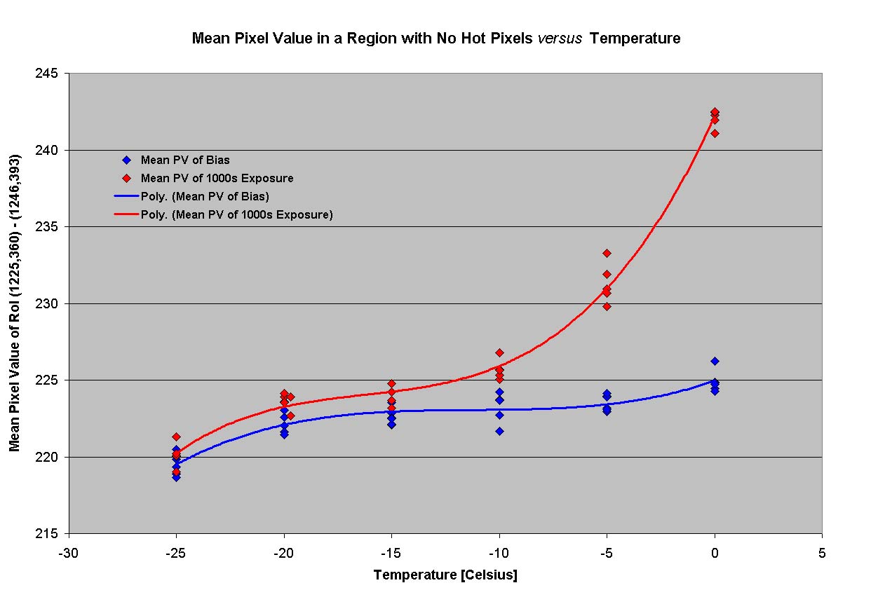
of images for analysis. The first thing I checked was the stability of the 532ws’ temperature. Dark current depends strongly on temperature, typically doubling every 6 degrees Celsius. If the CCD temperature oscillates around the set point temperature, dark frames have either more or less dark current the those taken at the nominal set point temperature. If you combine multiple dark frames at slightly different temperatures, in effect you’re hoping that the highs and lows will average out. Even if this is true, temperature oscillation contributes unwanted noise to your images. The QSI 532ws has a thermoelectric cooler. When you turn on the cooler, the camera cools rapidly, reaches the set point temperature, and then stays right at that temperature without oscillation above and below the set point. In checking over 500 dark frames, I found only two in which the CCD temperature did not equal the set point temperature, and then by only 0.2 degrees. I was quite satisfied with the stability of the 532ws’ temperature control. Dark frames I took in July worked perfectly with images that I shot in September. Dark current in the KAF-3200ME CCD proved more interesting than I expected. Dark current is a property of the CCD itself; aside from providing a stable thermal environment, the camera has nothing to do with the dark current. In the olden days, every pixel was a hot pixel. On the KAF-3200ME CCDs in the QSI cameras that I tested, the vast bulk of pixels had such low dark current that it was difficult to measure accurately. To get an accurate measurement of the dark current at a working temperature of -20 Celsius, I had to resort to extreme measures. I shot a sequence of 256 bias frames and 256 dark frames with an exposure of 60 seconds. Using AIP4Win’s Sigma-Clip Files function, I combined these into a master bias and a master dark frame, then subtracted the bias from the dark to create a master “60-second thermal frame.” A histogram (shown in Figure 5) produced by AIP4Win’s Pixel Tool shows that 99.8% of the pixels follow a Gaussian distribution, with a long-tailed distribution toward higher values. In this image of 3,124,848 pixels, one pixel had a pixel value 5995 ADU, 18 pixels had values >1000 ADU, 119 pixels had values >100 ADU, 2931 pixels had values >10 ADU, and 5982 pixels (0.2%) had values >3.5 ADU. The remaining 3,208,866 pixels lie in a Gaussian peak centered at 0.265 ADU, and of those pixels, 46% lay within ±0.5 ADU of the peak value. Converted to electron units, the hottest hot pixel had a dark current of 130 electrons/pixel/second, while the mean dark current for all pixels was 0.006 electrons/pixel/second. In practical terms, the dark current at -20C for 99.8% of the pixels on the CCD proved so small as to be negligible. Out of a total of 3.2 million pixels on this CCD, only ~6000 hot pixels displayed significant dark current. With this in mind, I examined the behavior of “good pixels.” I made sets of bias frames and accompanying dark frames with exposures up to 1000 seconds. Using the Pixel Tool in AIP4Win, I measured mean pixel values of the bias frames and the 1000-second dark frames in a region that was entirely free of hot pixels. The results are shown in Figure 6. Best-fit fourth-order curves represent these data well. At temperatures of -15C and lower, dark frames nearly match the values found in bias frames. Converting the difference between the 1000-second dark frames and the bias frames to dark current yields the following mean dark current for a region free of hot pixels:
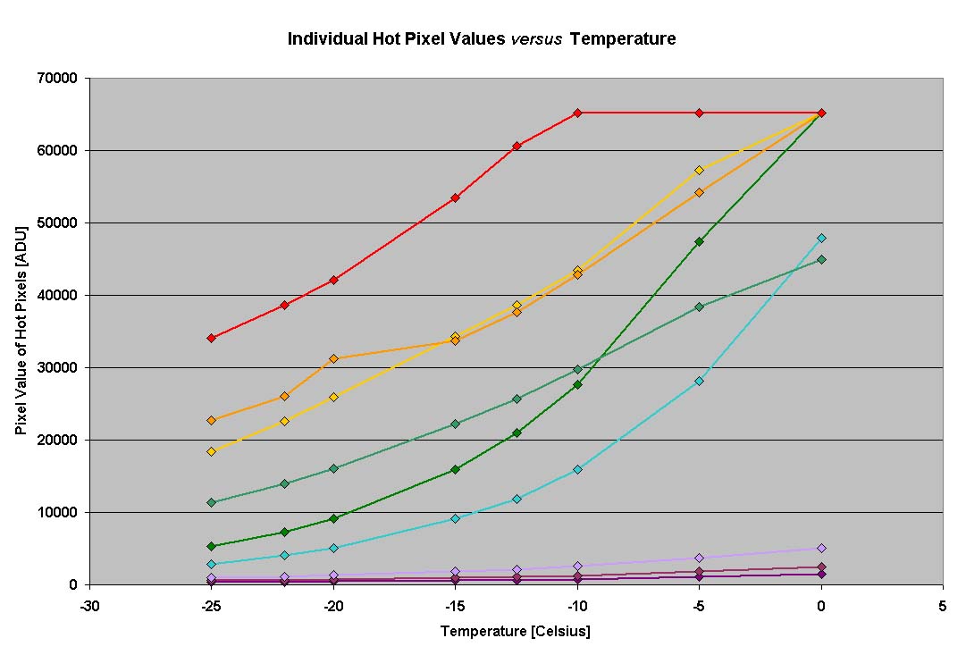
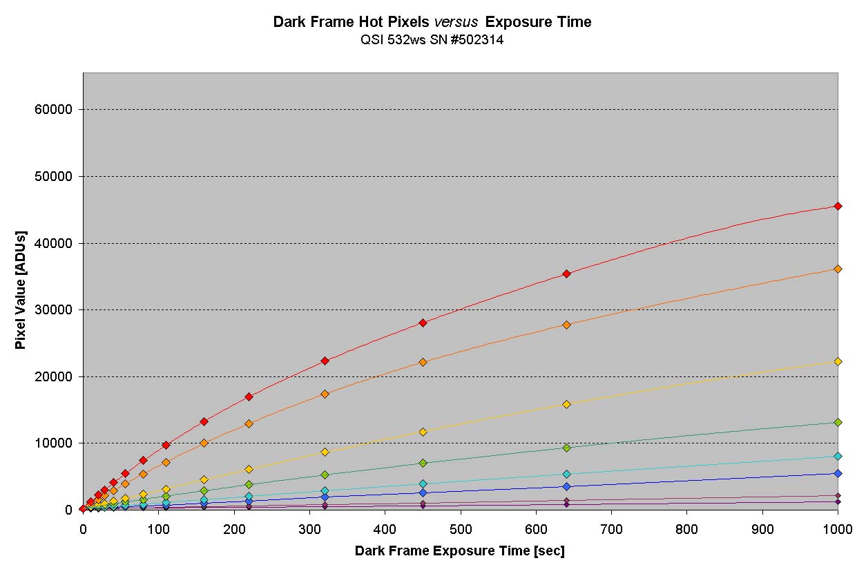
These figures are remarkably low, a dramatic tribute to Kodak’s mastery of CCD technology. We used to see performance like this with the Sony HAD CCDs; it appears that Kodak has excellent low-dark-current technology, too. From a practical viewpoint, these figures suggest that there’s no reason to run the QSI 532ws at temperatures lower than -20C to -25C because for 99.8% of the pixels on the CCD, the dark current nearly matches the bias, and is effectively zero. But what about the remaining 0.2% hot pixels? I wanted to know: How do the hot pixels on the KAF-3200ME behave? To sample the temperature behavior of hot pixels, I located six pixels that were either saturated or more than halfway to saturation at 0 Celsius, and three pixels with values below 5000 ADU. Using AIP4Win’s Pixel Tool, I measured the pixel value from a set of median-combined 1000-second exposures. Results are plotted in Figure 7. All hot pixels become “hotter” with higher temperature, but the rate of increase among the group of six appears to differ. Several curves cross—implying differing temperature coefficients—and, of course, some of the hot pixels reached saturation at 65535 ADU. Although too low to show well in the graph, the low value pixels appeared to behave with reasonable consistency. However, the unpredictable behavior the hottest hot pixels suggests that dark-frame subtraction may not work for a handful of hot pixels on each CCD. To sample the exposure time behavior of hot pixels, I used AIP4Win‘s Pixel Tool to measure a selection of hot pixels from a sequence of dark frames with exposures ranging from 10 seconds to 1000 seconds. The resulting plot, for a temperature of -20 Celsius, is shown in Figure 8. Although these curves appear quite well behaved, they are curves rather than straight lines; that is, the dark current of high-value hot pixels is non-linear with respect to exposure time. Among other things, these data suggest that with the KAF-3200ME (and quite possibly, other CCDs in the same device family), scaling dark frames linearly with time during dark-frame subtraction doesn’t correct a handful of hot pixels. This behavior can be countered by dithering the telescope pointing when taking images and using an algorithm such as sigma-clip to eliminate outlier values. The QSI 532ws camera provides a stable thermal environment for the KAF-3200ME. The CCD itself displays remarkably low dark current in ~99.8% of its pixels. Of the remaining 0.2% (~6000) hot pixels, it is likely that fewer than 100 of them respond erratically with temperature or non-linearly with exposure time. Used with care, standard calibration procedures can deal with this small number of high-value hot pixels. In any case, kudos to Kodak for making CCDs with such low dark current. |
||||||||||||||
Analysis of QSI 532ws Flat Frames |
||||||||||||||
| Flat frames
provide a window into a camera’s response to light,
specifically, they allow us to measure the linearity and
uniformity of the CCD. For the KAF-3200ME, Kodak
specifies nominal values for non-linearity and
non-uniformity of 1%, with maximum allowable values of 2%
non-linearity and 3% for non-uniformity. Although my
methods did not exactly match the test methods that Kodak
employs, my results suggest that QSI has succeeded in
squeezing every bit of performance possible from
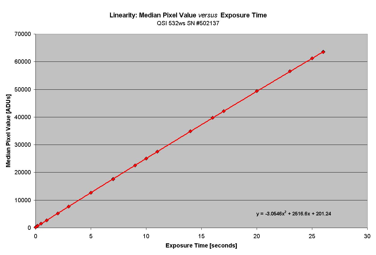
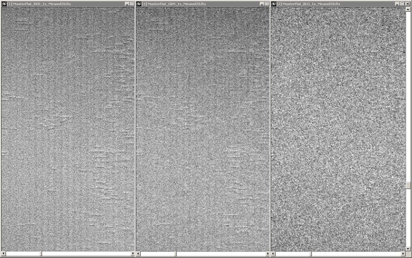
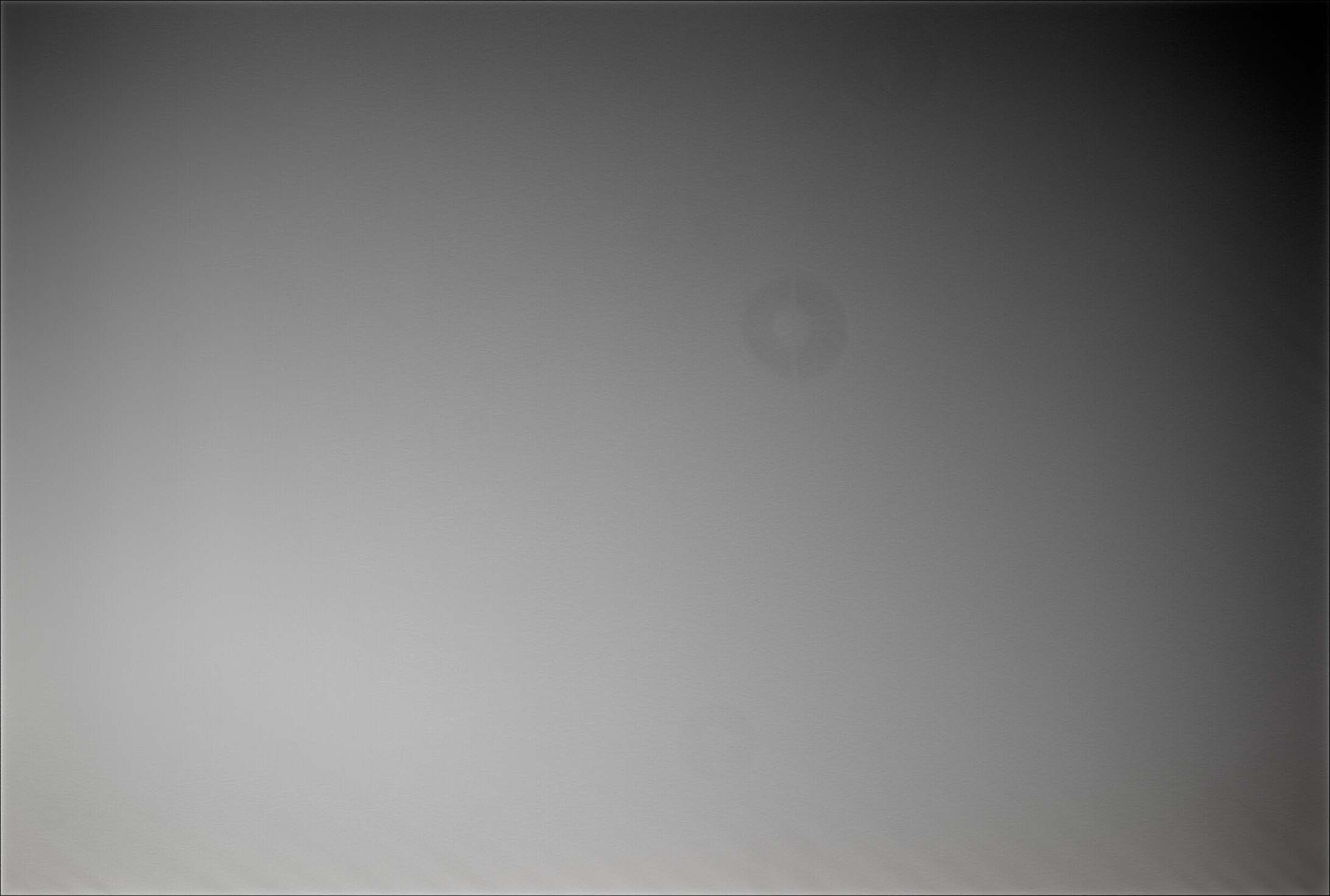
Kodak’s CCD. Linearity: Linear response means that the digital output from the CCD camera is strictly proportional to the incident light. CCDs with anti-blooming gates are intentionally made non-linear: they spill excess charge from pixels as they approach saturation. For astronomical science imaging, linear response is necessary for accurate photometry. In imaging, non-linear response in the CCD can lead to gradients in the image. However, the QSI 532ws test camera passed the linearity test with flying colors. In The Handbook of Astronomical Image Processing, we described a technique that can be used to determine linearity. To test the QSI 532ws, I wanted a technique that would more closely mimic taking real astronomical images. So I took a series of flat-field frames of increasing exposure with matching dark frames. After dark-subtraction, I measured the mean value of a uniform region in the center of flat-field image. This allowed me to test the camera’s linearity as if I were taking celestial images, which is what both aesthetic imagers and scientists really care about. For consistent results, I first had to make an extremely constant source of light. I tried an LED used with the constant-current circuit described in the Handbook, running from a 12-volt 5 amp-hour battery, but it declined by several percent over a two-hour period. Using a constant voltage circuit to run the constant-current circuit solved this problem. To guard against systematic brightness shifts, I made the exposures in rotating sets so that zero-exposure and maximum-exposure images occurred at regular intervals. Analysis of the images showed that no systematic shift in LED output occurred while the camera was taking data. In the setup that I used, the CCD saturated at roughly 26.5 seconds exposure. I set the minimum exposure to 0 seconds (i.e., bias frames), the maximum exposure to 26 seconds, and between the minimum and maximum, selected 20 exposure times from 0.1 seconds to 25 seconds. I used the camera’s shutter to time the exposures. I calibrated each image with its dark frame, then plotted the median value of the entire image against the exposure times. The response curve is shown in Figure 9. To the eye, this plot looks perfectly linear. But a linear least-squares fit reveals a non-linearity of +1% at 8 seconds exposure, and a minimum of -0.5% at 26 seconds exposure. Kodak specifies that the worst-case deviation from a straight-line fit between 2% and 90% of saturation is nominally 1%, so the system performance lies well within the Kodak’s specs. The QSI 532ws camera should be capable of 10-millimag photometry or better over its entire dynamic range. When I did a photometry run with the test camera, I achieved 5-millimag accuracy quite easily. Observing exoplanet transits should pose no problem for the QSI 532ws camera. Uniformity: Uniform response is crucial in making pictorial images. Can you imagine what would happen if one side of your CCD were more sensitive than the other side? Or if it were more sensitive to one color over another? You could get gradients and strange color effects in your images. I tested the color uniformity of the QSI 532ws, and once again, the camera and its CCD proved their merit. Kodak’s specification for uniformity requires a nominal 1% standard deviation from the mean value of a 128x128 sample when the CCD is illuminated uniformly. I wanted to verify that the KAF-3200ME was uniform in all standard LRGB colors. I made multiple flat-field frames using the Astronomik Type II R, G, B filters supplied with the test camera, and averaged them to make high-quality master flats. Figure 10 shows sample sections. When I measured sample blocks of the specified size, I found that one standard deviation was 0.25% for luminance flats, 0.32% for red-filtered flats, 0.35% for green-filtered flats, and 0.55% for blue-filtered flats. In other words, the CCD in the QSI 532ws camera bettered Kodak’s specification by two to four times. Departures from perfect uniformity took the form of short horizontal streaks and periodic vertical banding in the red and green flats, while the blue flat showed only the vertical banding. Since the pattern remains the same from frame to frame, it should be removed during routine flat-fielding. Although Kodak does not specify the uniformity of CCD with different color filters, it is an important consideration for making good-looking color images. Using AIP4Win’s Join colors Tool, I made a color image from flat-field frames. The resulting color image was almost perfectly gray. When I measured RGB values in a 24-bit color TIF image, they were usually identical, and seldom varied more than 1 ADU over the image. Figure 11 shows how neutral the RGB flat-frame image looks (yes, it's a color image!) Averaged over the whole image, the response of the CCD in blue light is approximately 0.1% higher in its center than the mean response, and around 0.2% lower around the edges in green and red. It was quite difficult to detect and measure such tiny non-uniformities; you would never detect them in normal astronomical imaging. |
||||||||||||||
Summary Evaluation Based on Test Images |
||||||||||||||
| Examination of bias frames, dark frames, and flat frames revealed that two QSI 532ws cameras and the KAF-3200ME CCDs in them performed to specification. I was unable to find any problem or noise source in the test images that could be attributed to any failing or fault in the QSI camera. | ||||||||||||||
Click here to read about the performance of the KAF-3200ME Image Sensor |
||||||||||||||
Stellar Photometry with the QSI 532ws |
||||||||||||||
| Measuring
stellar magnitudes is probably the most common type of
scientific observation undertaken by amateur astronomers.
It seemed natural, therefore, to evaluate the performance
of the QSI 532ws by making the light curve of an
interesting star. I selected the star BL Camelopardalis
because it’s reasonably easy at 13th
magnitude, it changes rapidly, and its northern location
means it’s possible to follow it for many hours. And
it’s easy to find: BL Cam is two-thirds of the way
from Polaris to the bright stars in Perseus, in the
middle of a prominent line of four stars. If you get the
middle two stars in your field of view, you’ve also
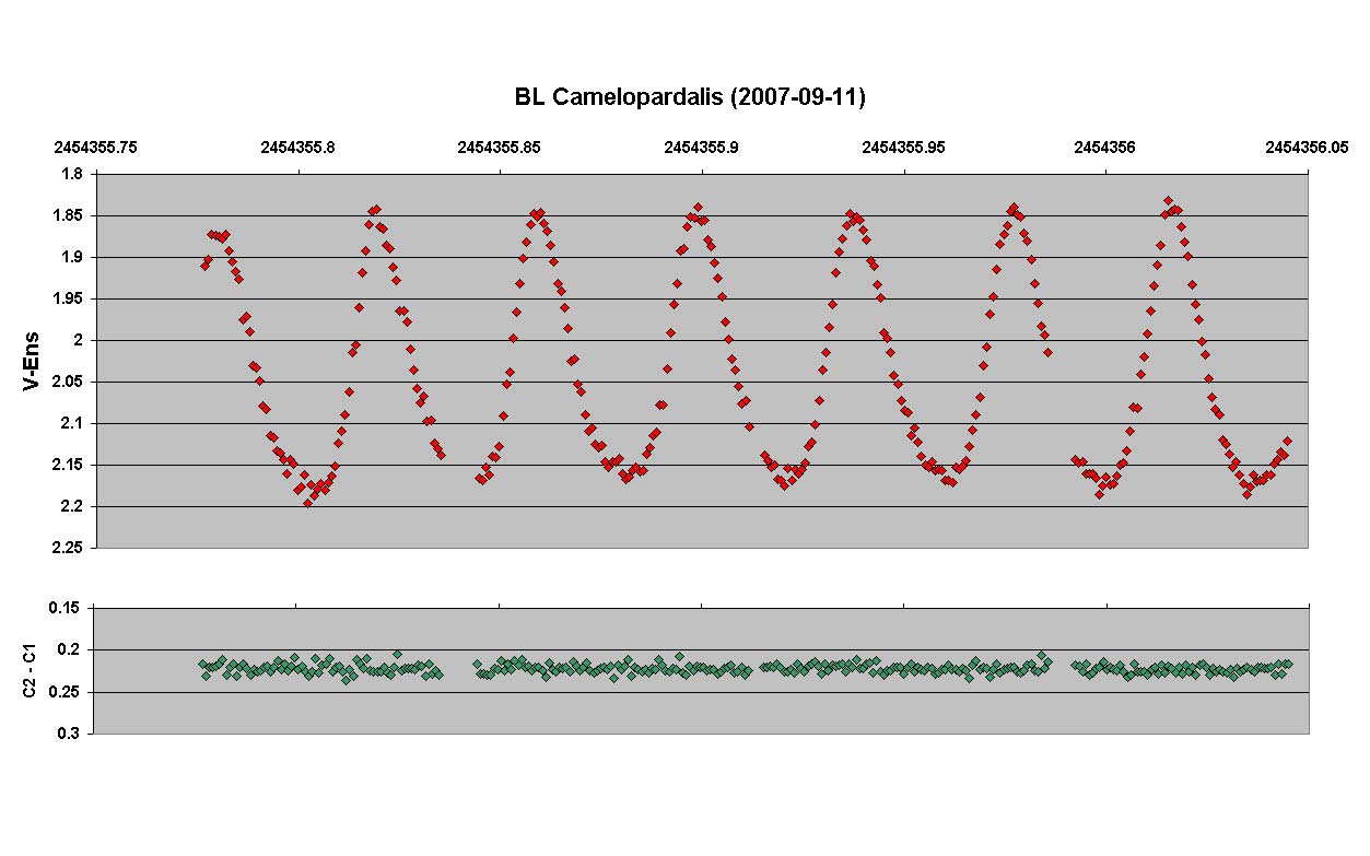
got BL Cam. I used the telescope and mount I normally use for imaging (Vixen R200SS 200 mm ƒ/4 Newtonian, Paracorr coma corrector, Byers 812 mount), and on two nights shot some ten hours worth of clear-filtered 60-second exposures. I auto-calibrated the images and performed aperture photometry using AIP4Win’s Multi-Image Photometry Tool. The longer of the two light curves is shown in Figure 15. The measured amplitude of variation is 0.35 magnitude and varies somewhat, and the period is under an hour. The curve looks as smooth as any of the light curves I found in the literature. The internal consistency of the data was excellent: the standard deviation of the differential magnitude between the comp and check star was 0.0055 magnitudes, in agreement with the expected error due to shot-noise and readout noise. While two nights of clear-filter photometry are hardly definitive, the QSI 532ws certainly did produce excellent light curves and magnitude uncertainty was consistent with the expected performance. |
||||||||||||||
Imaging with the QSI 532ws |
||||||||||||||
| Although the
month the test camera arrived was cloudy and rainy, when
the skies finally cleared, I set out to make test images
of astronomical objects. By then I had done enough work
with bias, dark, and flat frames that I had no doubt the
QSI camera would perform extremely well with astronomical
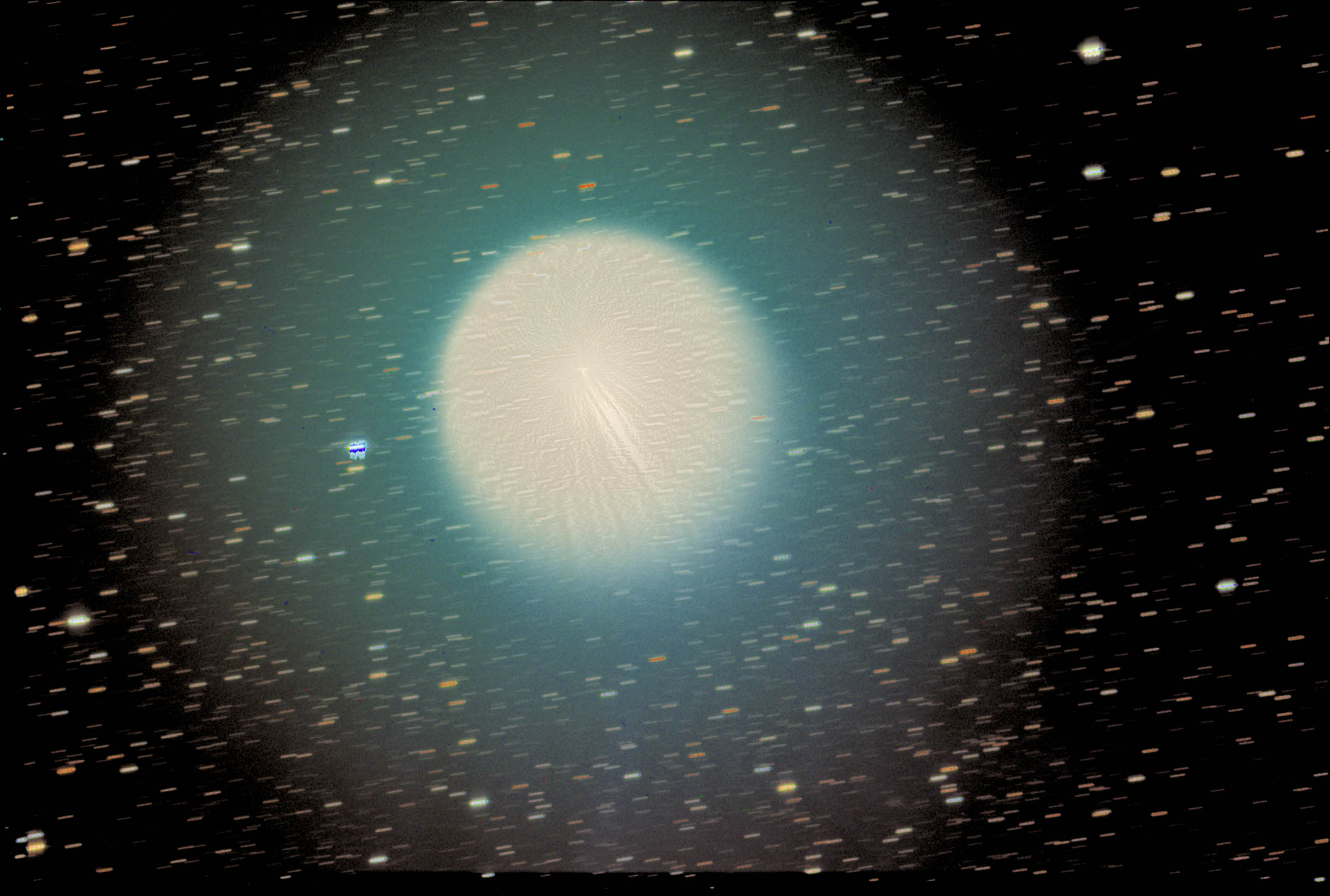
subjects. I used a Vixen R200SS 200 mm ƒ/4 Newtonian reflector with a Paracorr coma corrector on my faithful old Byers 812 mounting. The small pixels (6.8 microns square) turned out to be a good match for a fast Newtonian with a coma-corrector, and I must say that I was impressed with the performance of the Paracorr—nice round images right to the corner of the frame. I made sequences of 60-second exposures with the Astronomic LRGB Type IIc filters that come with the standard QSI 532ws camera kit, and stacked them with AIP4Win. In addition to images, I usually made 16 60-second dark frames, 16 light-box flats, and 16 flat-darks each night. Since the KAF-3200ME is a non-anti-blooming CCD, the bright stars in my images do exhibit blooming trails. Since my interests lean in the direction of astronomical science, I regard blooming trails as a small price to pay for high quantum efficiency and excellent linearity. At the telescope, the QSI 532ws was a pleasure to work with. I never needed to fight the camera to get good results; instead, it made my job easy. Its integral filter wheel and shutter are completely transparent to the observer—you set them as parameters in the acquisition software and the images get taken. My own QSI 532ws camera arrived about a month after I had sent the test camera back to QSI—just in time to catch Comet 17/P Holmes! The image in Figure 16 was made on November 2. I was able to perform many different analyses on the images, including cross-sectional brightness profiles, color-ratio images that revealed the color neutrality of the inner coma, the strong blue coloration of the outer coma, and the kinky and distorted tail. |
||||||||||||||
Design, Build Quality, and Overall Assessment |
||||||||||||||
| QSI asked me to
do a serious and demanding evaluation of their camera and
report any and all problems to them. When I got the
camera, I found it to be a real winner. Bias frames were
noise-free, cooling was rock stable, and all-around
performance was excellent. It has a compact footprint and
the workmanship is impressive. I ordered one for myself,
and when it arrived, I ran more tests on it, and found
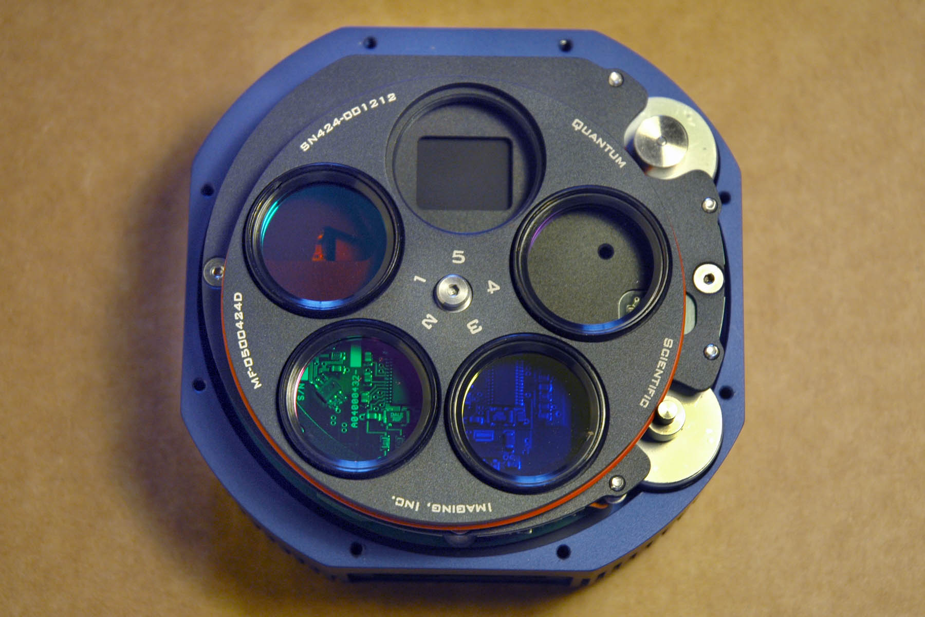
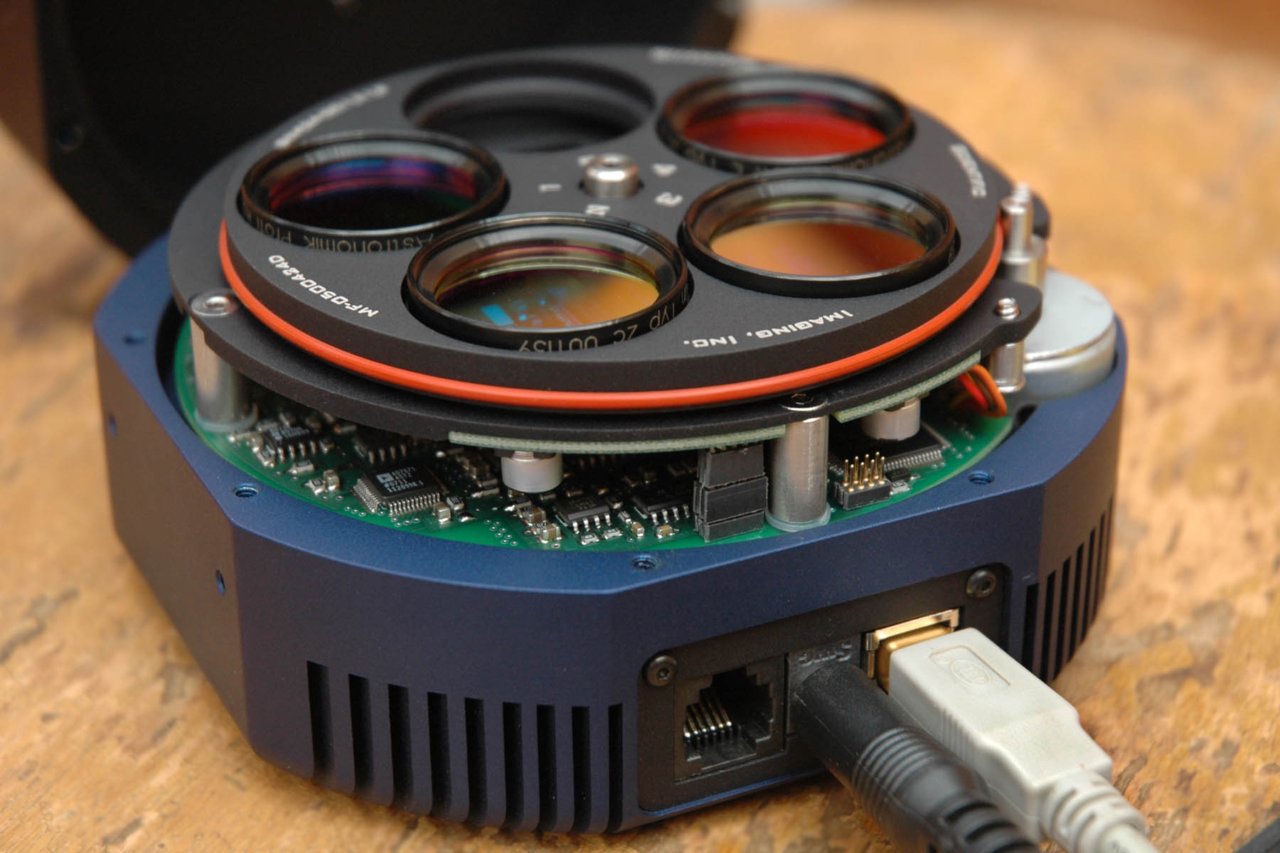
mine every bit as good as the test camera. The QSI 532ws met expectations when I tried CCD photometry of a variable star. When I made images of standard Messier and NGC objects, I got excellent LRGB results with total exposures sometimes under an hour. And when Comet 17/P Holmes appeared, my own QSI 532ws performed like a champ. I did not compare the QSI camera to other cameras in the amateur market. What I did was look for camera-generated noise sources, and check that the KAF-3200ME chip met or exceeded Kodak's specified performance levels. The camera tested out very clean, and the images met all of Kodak's specs. Although it's not relevant to science uses, the design of the 532ws is aesthetically pleasing. The camera is compact, rounded, and feels solid and good when you handle it. The machining is accurate, and parts fit very well. Changing the internal filter wheel is easy and takes just a few minutes. Figures 11 and 12show the tight integration of the internal filter wheel and shutter into the camera housing. The compact body design and short internal light path mean you can use the 532ws with optical systems as fast as ƒ/3.1 without vignetting using standard LRGB or narrow-band filters. The standard T-thread mount makes it equally easy to use on a telescope or with 35 mm camera lenses. Figure 17 and Figure 18 are close-up views of the camera with the front cover removed and the filter wheel and shutter revealed. I was impressed with the high sensitivity, the clean bias frames, the low dark current, the uniformity of the CCD’s response to light, and the smooth, reliable operation of the shutter and filter wheel. My overall assessment is that the QSI 532ws is a laboratory-quality camera that’s an outstanding value for amateur astronomers who demand top-notch imaging performance. |
||||||||||||||
Copyright © 2008 by Richard Berry |
||||||||||||||
Read about how I view performance testing a CCD camera. Examine some of the color images I made with the QSI 532ws. Return to Richard Berry's Home Page |
||||||||||||||